Introduction
You walk into a retail store. The moment you walk in, you notice several others are there to shop like you. Perhaps if something interests you, you may spontaneously choose to include it in your basket, but you have come to the store for a reason. Maybe you even have a list of things to buy in mind. That is, your shopping list is not purely random; it is constructed with purpose and the items included in it have meaningful economic relationships. But it’s not just you. Everyone shops with purpose.
This project aims to explore how people consume goods and what might influence the purchase of these goods by studying a large number of transactions from “The Complete Journey” dataset from Dunnhumby. The data includes over 275,000 baskets in total composed from any number of items from hundreds of unique commodities purchased by more than 2,500 households in over two years. This rich dataset offers ample opportunities to extract meaningful economic insights and perspectives such as:
- Which goods are the most purchased and which are the least purchased?
- What goods are frequently or rarely associated together?
- Do the income and/or the number of children have an influence on the purchases?
Let us take a peek at your basket
Studying quantities or sales value is not so interesting because different products can have wildly varying quantities and unit prices which may obscure our analysis. Instead, we focus on taking a peek at each basket in the transaction history and keeping track of product counts.
The number of items in a basket can range from 1 to 80 with an average size being 7 items. So most people buy under 10 products although there are certainly a few big shoppers from time to time. The product counts from all baskets allows us to discover products that have been purchased the most often:
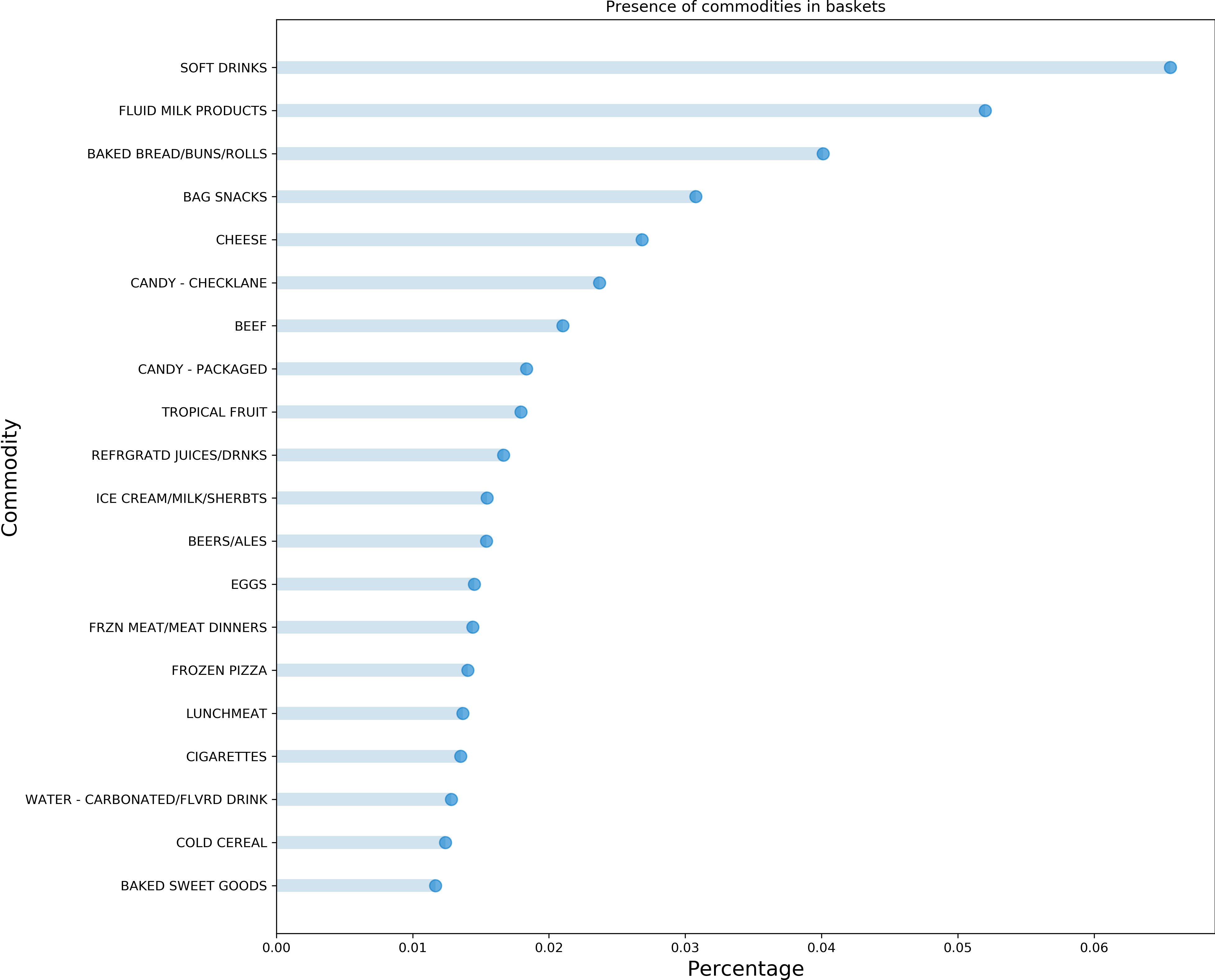
One would expect that products at the top of the ranking are cheap and basic goods. Indeed, we can see that the top 5 includes soft drinks, dairy products, bread, snacks and cheese, all of which are classic examples of inferior goods.
Interestingly, the most common bought product SOFT DRINKS is found in only 6% of the baskets. This result informs us that no products are systematically dominant in terms of purchases. This is a good indication of the inherent variety of purchases, and therefore we have a nice environment to study relationships between products.
Beyond just keeping track of product counts, we can keep track of the number of times a product is seen together with another product. This analysis leads to what we call the co-purchase matrix whose values indicate the total number of occasions that any pair of products were purchased together. This result can be most naturally visualized in the form of a network where each node represents a product and the weight of an edge is the value from the co-purchase matrix. By clicking on one node/product, we can visualize all other products with which this particular product have been purchased at least once in the past.
Note that the above network illustrates the co-purchase relationships from the study of the baskets, where the weights of the edges are the log-normalized number of times two products have been bought together. We only list the details of 15 most frequently co-purchased products in the pop-up box.
Visualizing with a network has the advantage of clearly seeing a product’s connections to the rest. It places the focus primarily on the existence of connections. Another great way to visualize product relationships is a heat map, which presents the advantage of visualizing the weight of the connections while also highlighting the sparsity of the overall network at the same time. Below is an interactive heat map where the values are again the log-normalized number of times two products have been bought together.
In the symmetric matrix above where the y- and x-axis represent the indices of the unique products, two products stand out: SOFT DRINKS and FLUID MILK PRODUCTS. These correspond to the particularly bright columns (or rows) in the heat map. Despite the fact that a product appears at best in only 6% of the baskets, these two products have a strong co-purchase association with nearly all other products in the retailer.
The network now unlocks a number of interesting graph analysis for us. In particular, we focused on identifying bridges. A bridge is an edge which, when removed, creates two disconnected components in the network. In our product network, bridges offer an interesting economic insight in its own way because by removing them we were able to isolate products which have only been co-purchased with only a single other product. The bridges are visualized in the following interactive plot.
Below are five most interesting bridges we found in our product network. The product on the left is the isolated product and the product on the right was the only product it was ever purchased with:
FUEL→CIGARETTESROSES→GREETING CARDS/WRAP/PARTY SPLYSANDWICHES→SOFT DRINKSCHIPS&SNACKS→SOFT DRINKSSYRUPS/TOPPINGS→ICE CREAM/MILK/SHERBTS
As we can see, these bridges are quite intuitive. For example, when people come to buy FUEL (gas), it is often the only thing they buy, or if bought with anything else, it is always purchased with CIGARETTES. Similarly, CHIPS&SNACKS are always seen together with SOFT DRINKS if it isn’t the only thing in the basket.
Now, the central aspect of the study of the product network is to identify economically intuitive groups or communities of products based on the co-purchase occasions. However, prior to this final analysis, we would like to explore a few more potentially important factors that might influence purchases decisions, and thus develop a more comprehensive economic understanding. To this end, we diverge briefly in the next section to analyze household income and number of children only so that its insights can ultimately be combined to the product analysis in the network.
Do children and household income matter?
Household income in the dataset largely falls into 12 brackets from “under 15K” to “200-249K” with the median income at approximately $29,500. It also turns out that roughly 64% of the households do not have children, so we can see that the retailer is mainly visited by low-income family units with no dependents.
One approach to studying the effect of household income on consumption patterns is to analyze the weekly average expenditures per product per household in each income bracket to identify any statistically significant differences between brackets. A similar analysis can be conducted in each number-of-children bracket which varies from “0” to “3+”. Below are three most correlated products with income and number of children respectively.
The weekly expenditures are normalized by max-scaling in each product since what matters is the degree of correlation rather than the actual weekly expenditure per se. Weekly expenditures are bound to vary significantly from product to product due to the differences in their unit prices and therefore obscure the scale on the y-axis significantly.
Products such as SUNTAN and HOME HEALTH CARE are luxury products and are expected to be correlated with income. SUNTAN, for example, correlates well with the number of occasions of vacation while HOME HEALTH CARE products can include personal care, drugs, and medical equipment. SNACK NUTS is a more surprising result, but the fact that their prices are typically on the higher-end relative to other snacks may help explain this.
It appears logical that HALLOWEEN, which spans anything from decorating lights to costume accesories, is strongly correlated with the number of children. Likewise, GLASSWARE & DINNERWARE is expected to be positively correlated with the size of the family unit as they need more dishes at home, or perhaps also because children tend to break plates easily.
But which of these items is strongly correlated with both household income and the number of children? Which ones are only closely related to either one exclusively? The mapping of some of the most interesting products in these two dimensions is demonstrated below.
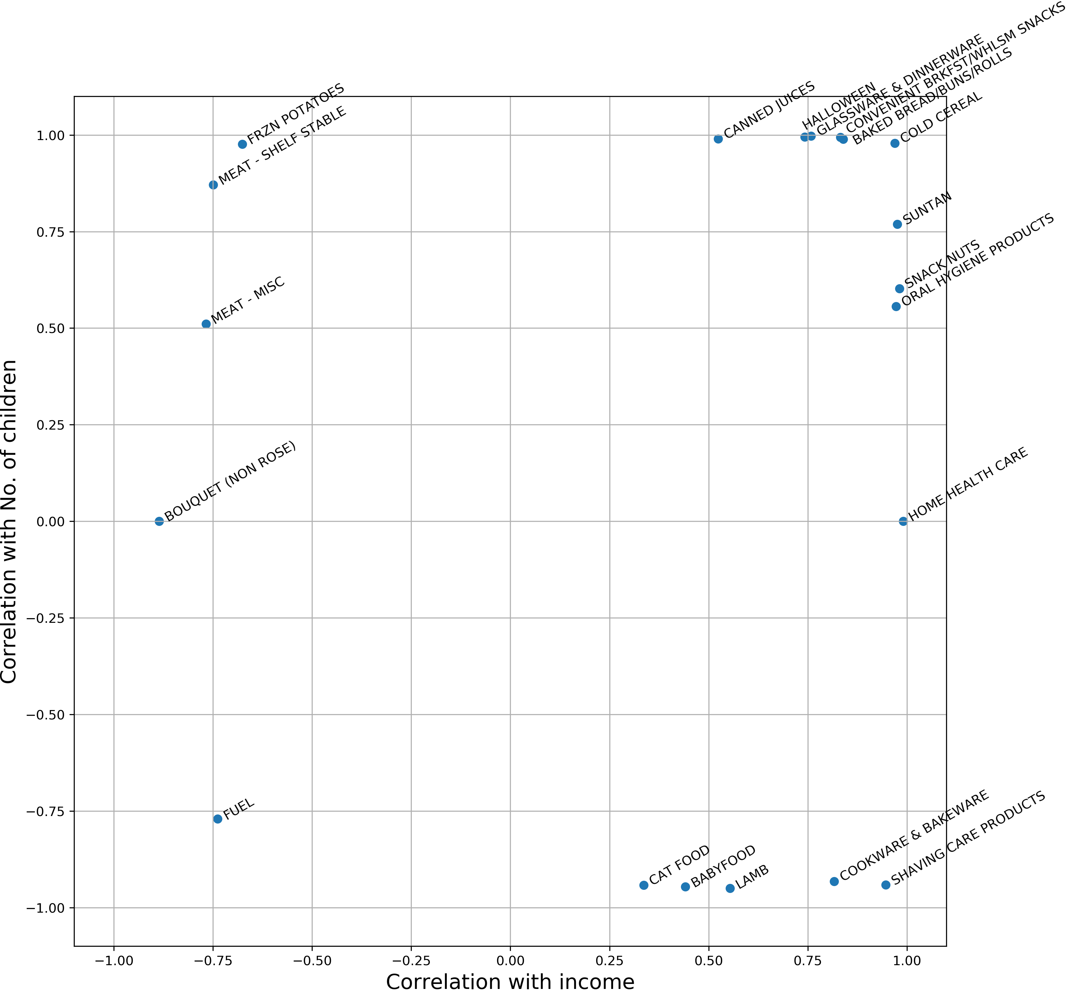
The examples at the corners of this spectrum may shed light on meaningful relationships between purchase decisions and the two economic factors. For instance, FRZN POTATOES and MEAT - SHELF STABLE (i.e. canned goods typically designed to remain unspoiled for a long time) are negatively correlated with income as these are typical inferior goods. Furthermore, it is sensible they are positively correlated with the number of children at the same time. Furthermore, food products such as BAKED BREAD/BUNS/ROLLS and COLD CEREAL are positively correlated with both income and number of children, which is again reasonable.
As a final remark, we point to some unintuitive results in this plot such as the negative correlation of BABY FOOD with the number of children. The fact that BABY FOOD is among the 30 products with the lowest backet counts as well as co-purchase counts might help justify this counter-intuitive finding since this implies there aren’t enough samples of it in our data.
“Clique on the link”
The final task remains at hand: linking the economic factors we have just analyzed to the communities of products we may potentially discover in our product network. One way to detect these communities is by identifying cliques within the network (hence the title “clique on the link”).
A group of products is a clique if there exists at least one co-purchase count between every pair of products. We can expect that the products in the same clique are therefore complementary goods whose sales tend to move together. But could the relationship between a household’s weekly expenditure and its income somehow depend on the cliques? Below, you will find an interactive plot in which you have the possibility to select some cliques and highlight them in the product network.
One important aspect of our product network is that it is close to an “ego-network” where many products are directly connected to one or two products, namely SOFT DRINKS or FLUID MILK PRODUCTS. Keeping this in mind, we turn our attention more towards items in the cliques other than these two items to discover meaningful complementary relationships. Indeed, as you may have already noticed, we have some interesting cliques that are intuitive economically:
- Clique “Household items”:
PAPER TOWELS,DISHWASH DETERGENTS,HOUSEHOLD CLEANING NEEDS,BROOMS AND MOPS - Clique “Alcohol”:
BEERS/ALES,IMPORTED WINE,DOMESTIC WINE,CHEESE - Clique “Food mix #1”:
ORGANICS FRUIT & VEGETABLES,CHEESE,BEEF,REFRIGERATED - Clique “Food mix #2”:
SALAD MIX,PROCESSED,TOMATOES,BERRIES - Clique “Festivities”:
CHRISTMAS SEASONAL,GREETING CARDS/WRAP/PARTY SUPLY,CANDY - PACKAGED,CANDY - CHECKLANE - Clique “Hygiene products”:
ORAL HYGIENE PRODUCTS,MAKEUP AND TREATMENT,HAND/BODY/FACIAL PRODUCTS,HAIR CARE PRODUCTS,CANDY - PACKAGED
From these discoveries, one can quite intuitively surmise that products with the same general purpose with slightly differing uses or functionalities are complementary. In other words, the cliques above tell us that the sales of household items for doing chores, of alcoholic drinks, of common vegetable and meats, of festivities, and of hygiene products increase together.
What’s more, all of these cliques are found to have statistically significant effect on the correlation between weekely expenditure and household income. Put differently, weekly spending in general appears to be positively correlated with household income when looking only at the products in these cliques. A prime example is the clique “Alcohol”; the more the household income, the more the spending on alcoholic drinks seems to be.
Conclusion
Purchase decisions are dfficult to generalize and are not always intuitive. Retailers constantly bombard consumers with tactics for impulse buying which may obscure fundamental economic relationships in a backet of goods, let alone that considerable number of people do tend to buy on the fly. However, with data collected over a sufficiently long time span and analyzed over a large number of unique baskets of goods from many households, we can still gain valuable insights into the inherent consumption patterns.
We have verified that many of these patterns are economically intuitive. Soft drinks are most commonly seen across all baskets. Certain products such as milk are remarkably connected and co-purchased with many other products. People stop for gas and that’s often the only thing they stop for; otherwise, they tend to buy cigarettes while they have time. Bouquets are only bought with greeting cards because it makes sense that you would write a few kind, loving words to whom you will present the pretty flowers. Household chores-related things are tightly grouped together in terms of co-purchase, so are alcoholic drinks, and so are common vegetables and meats.
An interesting extension of this study can be about how to leverage these findings for business improvements. Are items in the stores organized and arranged in accordance with these relationships? Can sales increase even more by arranging items in the same clique in a more presentable, easier-to-find way? For products that are rarely associated with anything and also has low sales on its own, could the business actually consider putting these items out of stock to reduce overall costs? While in this project we mainly explored interesting economics at play, it is clear that much of these findings can potentially be incorporated into real-life decisions.